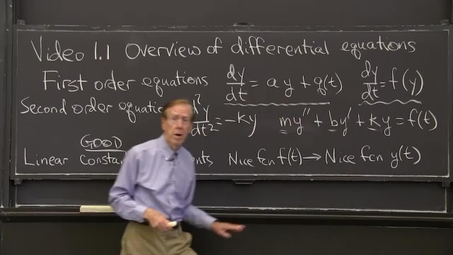
Linear equations include dy/dt = y, dy/dt = –y, dy/dt = 2ty. The equation dy/dt = y*y is nonlinear.
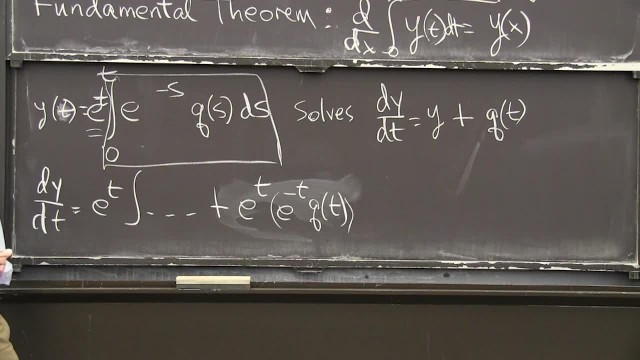
The sum rule, product rule, and chain rule produce new derivatives from the derivatives of x^n, sin(x) and e^x. The Fundamental Theorem of Calculus says that the integral inverts the derivative.
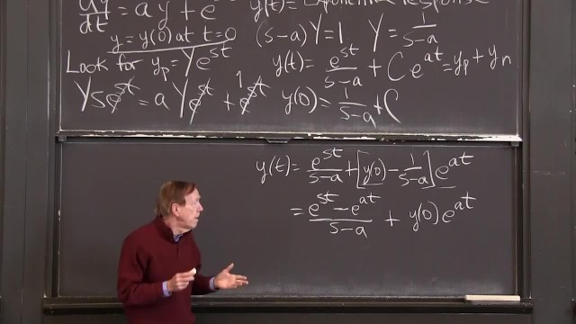
With exponential input, e^st, from outside and exponential growth, e^at, from inside, the solution, y(t), is a combination of two exponentials.
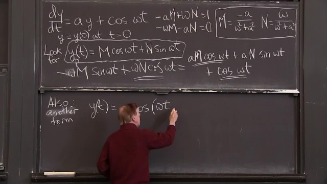
An oscillating input cos(ωt) produces an oscillating output with the same frequency ω (and a phase shift).
To solve a linear first order equation, multiply each input q(s) by its growth factor and integrate those outputs.
A unit step function jumps from 0 to 1. Its slope is a delta function: zero everywhere except infinite at the jump.
For linear equations, the solution for f = cos(ωt) is the real part of the solution for f = e^iωt. That complex solution has magnitude G (the gain).
The integrating factor e^at multiplies the differential equation, y’=ay+q, to give the derivative of e^-aty: ready for integration.
The integral of a varying interest rate provides the exponent in the growing solution (the bank balance).
When –by^2 slows down growth and makes the equation nonlinear, the solution approaches a steady state y(∞) = a/b.
Steady state solutions can be stable or unstable – a simple test decides.
Separable equations can be solved by two separate integrations, one in t and the other in y. The simplest is dy/dt = y, when dy/y equals dt. Then ln(y) = t + C.
For the oscillation equation with no damping and no forcing, all solutions share the same natural frequency
With forcing f = cos(ωt), the particular solution is Y*cos(ωt). But if the forcing frequency equals the natural frequency there is resonance
With constant coefficients in a differential equation, the basic solutions are exponentials e^st. The exponent s solves a simple equation such as As^2 + Bs + C = 0.
The impulse response g is the solution when the force is an impulse (a delta function). This also solves a null equation (no force) with a nonzero initial condition.
Resonance occurs when the natural frequency matches the forcing frequency — equal exponents from inside and outside.
A damped forced equation has a particular solution y = G cos(ωt – α). The damping ratio provides insight into the null solutions.
Current flowing around an RLC loop solves a linear equation with coefficients L (inductance), R (resistance), and 1/C (C = capacitance).
With constant coefficients and special forcing terms (powers of t, cosines/sines, exponentials), a particular solution has this same form.
This method is also successful for forces and solutions such as (at^2 + bt +c) e^st: substitute into the equation to find a, b, c.
Combine null solutions y1 and y2 with coefficients c1(t) and c2(t) to find a particular solution for any f(t).
Transform each term in the linear differential equation to create an algebra problem. You can then transform the algebra solution back to the ODE solution, y(t).
The second derivative transforms to s^2Y and the algebra problem involves the transfer function 1/ (As^2 + Bs +C).
When the force is an impulse δ (t), the impulse response is g(t). When the force is f(t), the response is the “convolution” of f and g.
The direction field for dy/dt = f(t,y) has an arrow with slope f at each point t, y. Arrows with the same slope lie along an isocline.
Solutions to second order equations can approach infinity or zero. Saddle points contain a positive and also a negative exponent or eigenvalue.
Imaginary exponents with pure oscillation provide a “center” in the phase plane. The point (y, dy/dt) travels forever around an ellipse.
A second order equation gives two first order equations for y and dy/dt. The matrix becomes a companion matrix.
A critical point is a constant solution Y to the differential equation y’ = f(y). Near that Y, the sign of df/dy decides stability or instability.
With two equations, a critical point has f(Y,Z) = 0 and g(Y,Z) = 0. Near those constant solutions, the two linearized equations use the 2 by 2 matrix of partial derivatives of f and g.
Two equations y’ = Ay are stable (solutions approach zero) when the trace of A is negative and the determinant is positive.
A box in the air can rotate around its shortest and longest axes. Around the middle axis it tumbles wildly.
An m by n matrix A has n columns each in Rm. Capturing all combinations Av of these columns gives the column space – a subspace of Rm.
Vectors v1 to vd are a basis for a subspace if their combinations span the whole subspace and are independent: no basis vector is a combination of the others. Dimension d = number of basis vectors.
A matrix produces four subspaces – column space, row space (same dimension), the space of vectors perpendicular to all rows (the nullspace), and the space of vectors perpendicular to all columns.
A graph has n nodes connected by m edges (other edges can be missing). This is a useful model for the Internet, the brain, pipeline systems, and much more.
The incidence matrix A has a row for every edge, containing -1 and +1 to show the two nodes (two columns of A) that are connected by that edge.
The eigenvectors x remain in the same direction when multiplied by the matrix (Ax = λx). An n x n matrix has n eigenvalues.
A matrix can be diagonalized if it has n independent eigenvectors. The diagonal matrix Λis the eigenvalue matrix.
Diagonalizing A = VΛV–1 also diagonalizes An = VΛnV–1.
dy/dt = Ay contains solutions y = eλtx where λ and x are an eigenvalue / eigenvector pair for A.
The shortest form of the solution uses the matrix exponential y = eAt y(0). The matrix eAt has eigenvalues eλt and the eigenvectors of A.
A and B are “similar” if B = M-1AM for some matrix M. B then has the same eigenvalues as A.
Symmetric matrices have n perpendicular eigenvectors and n real eigenvalues.
An oscillation equation d2y/dt2 + Sy = 0 has 2n solutions (sines and cosines). Solutions use the eigenvectors of S.
A positive definite matrix S has positive eigenvalues, positive pivots, positive determinants, and positive energy vTSv for every vector v. S = ATA is always positive definite if A has independent columns.
The SVD factors each matrix A into an orthogonal matrix U times a diagonal matrix Σ (the singular value) times another orthogonal matrix VT: rotation times stretch times rotation.
A second order equation can change its initial conditions on y(0) and dy/dt(0) to boundary conditions on y(0) and y(1).
The partial differential equation ∂2u/∂x2 + ∂2u/∂y2 = 0 describes temperature distribution inside a circle or a square or any plane region.
A Fourier series separates a periodic function F(x) into a combination (infinite) of all basis functions cos(nx) and sin(nx).
Even functions use only cosines (F(–x) = F(x)) and odd functions use only sines. The coefficients an and bn come from integrals of F(x) cos(nx) and F(x) sin(nx).
Inside a circle, the solution u(r, θ) combines rn cos(nθ) and rn sin(nθ). The boundary solution combines all entries in a Fourier series to match the boundary conditions.
The heat equation ∂u/∂t = ∂2u/∂x2 starts from a temperature distribution u at t = 0 and follows it for t > 0 as it quickly becomes smooth. The heat equation ∂u/∂t = ∂2u/∂x2 starts from a temperature distribution u at t = 0 and follows it for t > 0 as it quickly becomes smooth.
The wave equation ∂2u/∂t2 = ∂2u/∂x2 shows how waves move along the x axis, starting from a wave shape u(0) and its velocity ∂u/∂t(0).